Diffusion Models Notes
Diffusion Models (Part 1)
“The essential idea, inspired by non-equilibrium statistical physics, is to systematically and slowly destroy structure in a data distribution through an iterative forward diffusion process. We then learn a reverse diffusion process that restores structure in data, yielding a highly flexible and tractable generative model of the data.”
— Deep Unsupervised Learning using Nonequilibrium Thermodynamics
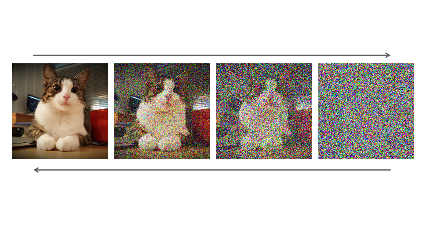
Figure: Overview of the forward and reverse diffusion process. Source: NVIDIA Developer Blog
Motivation
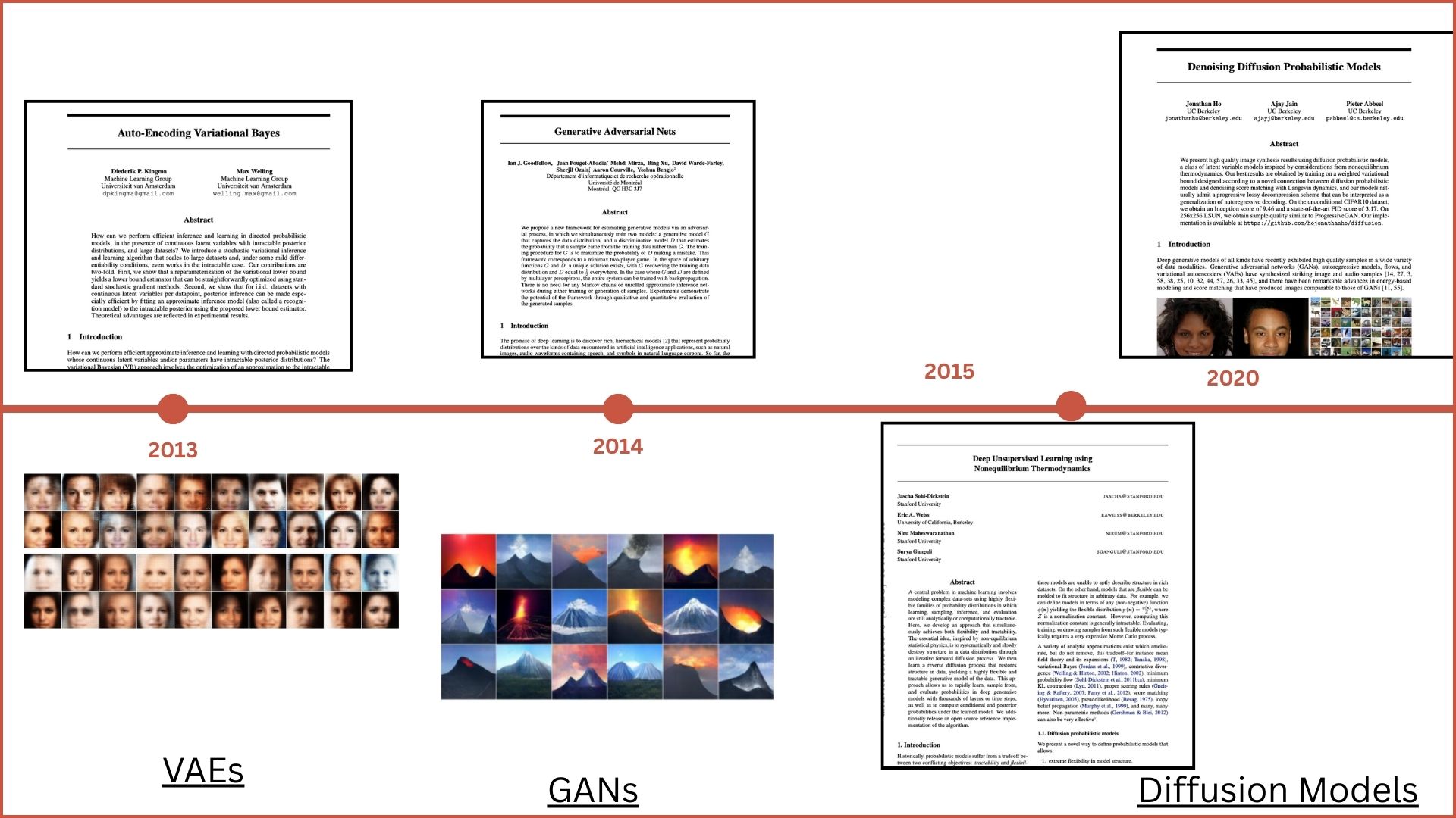
We are currently in the context of image-generation models. Previously, we have seen VAEs and GANs. These models are stepping stones to diffusion models, which are now the state-of-the-art for high-quality, diverse image generation.
First came VAEs (Variational Autoencoders), which learn a probabilistic mapping between input data and a latent representation using an encoder-decoder structure. They are effective because they allow for smooth latent space interpolation and tractable inference using variational methods. However, their main drawback is that the generated images tend to be blurry, as the decoder often optimizes for pixel-wise reconstruction loss (typically L2), which penalizes sharp details. VAEs suffer at generating high-quality images.
Then came GANs (Generative Adversarial Networks), which pit a generator network against a discriminator in a minimax game. A generator tries to create images to fool a discriminator and gets better at this objective throughout training. GANs are capable of generating sharp, realistic images and have had a huge impact on image synthesis. They are effective because the adversarial loss encourages outputs that are indistinguishable from real data. However, GANs are notoriously difficult to train due to instability, mode collapse (where the generator produces limited diversity), and sensitivity to hyperparameters. This means GANs can fail to represent the diversity of a dataset.
Then Diffusion Models emerged, gaining traction with the introduction of Denoising Diffusion Probabilistic Models (DDPMs), first proposed by Ho et al. in their 2020 paper “Denoising Diffusion Probabilistic Models.” These models work by learning to reverse a gradual noising process applied to data, effectively training a model to denoise inputs over many time steps.
Diffusion models are powerful because they combine the stability of likelihood-based models like VAEs with the high sample quality of GANs. They are trained using a simple denoising loss and are robust to mode collapse. Their main drawback is the slow sampling time, as generating an image requires hundreds to thousands of denoising steps. Nevertheless, newer approaches like DDIMs and Denoising Score Matching aim to speed up this process.
High-Level Overview
A diffusion model consists of two main components: the forward process and the reverse process.
- In the forward process, we gradually add noise to an image over several steps, eventually transforming it into pure noise.
- In the reverse process, a neural network is trained to systematically denoise this noisy image, step-by-step, until it reconstructs a high-quality, realistic image.
This iterative approach enables the model to learn a powerful generative mapping from noise to data. Thus, we want to learn how to generate any image from Gaussian noise, or learn de-noising patterns.
Forward Process
In the forward (diffusion) process we corrupt a clean sample \(x_0\) by adding Gaussian noise over T timesteps, producing a sequence \({x_t}_{t=1}^{T}\).
One‑step transition
For each timestep \(t = 1,\dots,T\) we draw fresh noise \(\varepsilon_t \sim N(0, I)\) and set
where \(\beta_t \in (0,1)\) is the variance schedule.
Define
Using the re‑parameterisation
we see that each step injects additional noise while shrinking the signal.
Closed‑form sample from \(x_0 \rightarrow x_t\)
Recursively expanding the expression above gives
where \(\varepsilon \sim N(0,I)\) absorbs the linear combination of all previous \(\varepsilon_s\).
Hence
This closed‑form expression lets us sample any noisy timestep in one shot, avoiding an explicit \(1 \to 2 \to \cdots \to t\) simulation.
Practical note
The schedule \({\beta_t}\) must keep \(\beta_t\ll 1\) to prevent the variance from exploding; common choices are a linear or cosine schedule (Ho et al., 2020; Nichol & Dhariwal, 2021).
Derivation adapted from
T. Ho, J. Salimans, et al., “Denoising Diffusion Probabilistic Models,” 2020.
Choosing the noise schedule
Linear schedule (original DDPM):
In the original DDPM, the noise schedule is chosen so that \(\beta_t\) increases linearly over time. Since
$$ \alpha_t = 1 - \beta_t, $$\(\alpha_t\) decreases as \(t\) increases. Intuitively, each forward step keeps slightly less of the original image signal and adds slightly more Gaussian noise. Early timesteps only mildly corrupt the image, while later timesteps push \(x_t\) closer to pure noise.
Diffusion Models: Reverse Process
What is the Reverse Process?
The reverse process is the generative part of diffusion models.
- It learns to undo the noise added during the forward (noising) process.
- Goal: Generate a sample that resembles the original data by reversing the Markov chain.
Idea
- We destroy data with Gaussian noise in the forward process.
- Now, we want to learn how to denoise step-by-step to recover the original image.
- Since the forward process is a Markov chain, we assume the reverse can also be modeled as a Markov chain, but in reverse.
Since the forward process defines a Markov chain \(q(x_{1:T} \mid x_0)\), the reverse process is modeled as a parameterized Markov chain:
where \(p(x_T) = N(x_T; 0, I)\) and each transition is modeled as a Gaussian:
Mathematical Formulation
- (Recall) forward process:
- Ideal reverse process:
- At inference time, we don’t have access to \(x_0\), so we:
- Train a model \(\epsilon_\theta(x_t, t)\) to predict the noise.
Learning the Reverse
We use the reparameterization:
Then optimize this loss (this is simplified from ELBO):
Training Objective via Variational Inference
We want to maximize the data log-likelihood:
This is intractable, so we use variational inference to derive a lower bound using the forward process \(q(x_{1:T} \mid x_0)\) as the variational distribution. Applying Jensen’s inequality gives the Evidence Lower Bound (ELBO):
Using the Markov factorization:
Rewriting the full form (Ho et al., 2020) leads to:
The KL terms compare the true reverse posterior with the learned reverse model.
Architecture
Commonly used model: U-Net (more on this in next set of notes)
Captures both local and global information
Time conditioning via sinusoidal positional embeddings
Often includes residual connections and self-attention layers
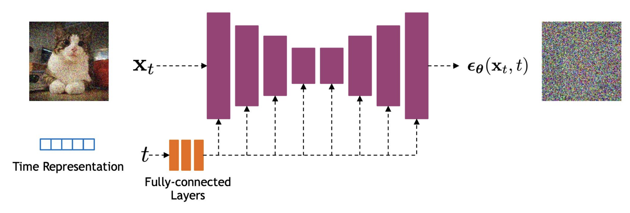 [Figure: From CS 4782 Class Notes 2025]
Inference
- Start from \(x_T \sim N(0,I)\)
- At each step, denoise using the trained model:
Summary
The reverse process generates new samples by reversing noise.
It requires training a neural network to approximate the denoising steps.
The loss function is mean squared error between predicted and actual noise.
This process is repeated iteratively from pure noise to produce coherent outputs.
Training Objective:
Our ultimate goal is to maximize the likelihood of the data, i.e.:
However, this is often intractable (no efficient algorithm to solve it). So, as in VAEs, we use the Evidence Lower Bound (ELBO) as a surrogate objective:
We can bound the likelihood with the ELBO (recall VAEs) such that
Specifically, for diffusion models, we write the ELBO in terms of the forward and reverse diffusion processes.
Where the first term ins the reconstruction term, the second is the prior matching term, and the last is the denoising matching term.
Explanation of Terms
- Reconstruction Term:
This encourages the reverse process to reconstruct the original input \(x_0\) from a noisy version \(x_1\). It’s similar to the reconstruction loss in a VAE.
- Prior Matching Term:
This penalizes the difference between the noisy endpoint distribution and the standard normal prior. Ideally, \(x_T\) should resemble pure Gaussian noise.
- Denoising Matching Term:
This ensures that at each timestep, the model learns to denoise \(x_t\) into a distribution that matches the true reverse of the forward process.
Simplified Loss for Training
Ho et al. propose predicting the noise \(\varepsilon\) added at each step, and minimizing the expected squared error:
where
This loss is derived from the KL terms in the ELBO under the assumption that the variance is fixed and only the mean is learned.
Why Use the ELBO?
The ELBO provides a tractable surrogate for the intractable log-likelihood \(\log p_\theta(x_0)\).
By maximizing this lower bound, we ensure:
- We are learning a model whose reverse process approximates the true posterior trajectory from \(x_T\) to \(x_0\).
- The training is stable and grounded in variational inference.
- The model generates samples that match the data distribution when denoised from pure noise.
This theoretical framework connects diffusion models to well-established probabilistic principles, enabling principled training and evaluation.
Training Algorithm
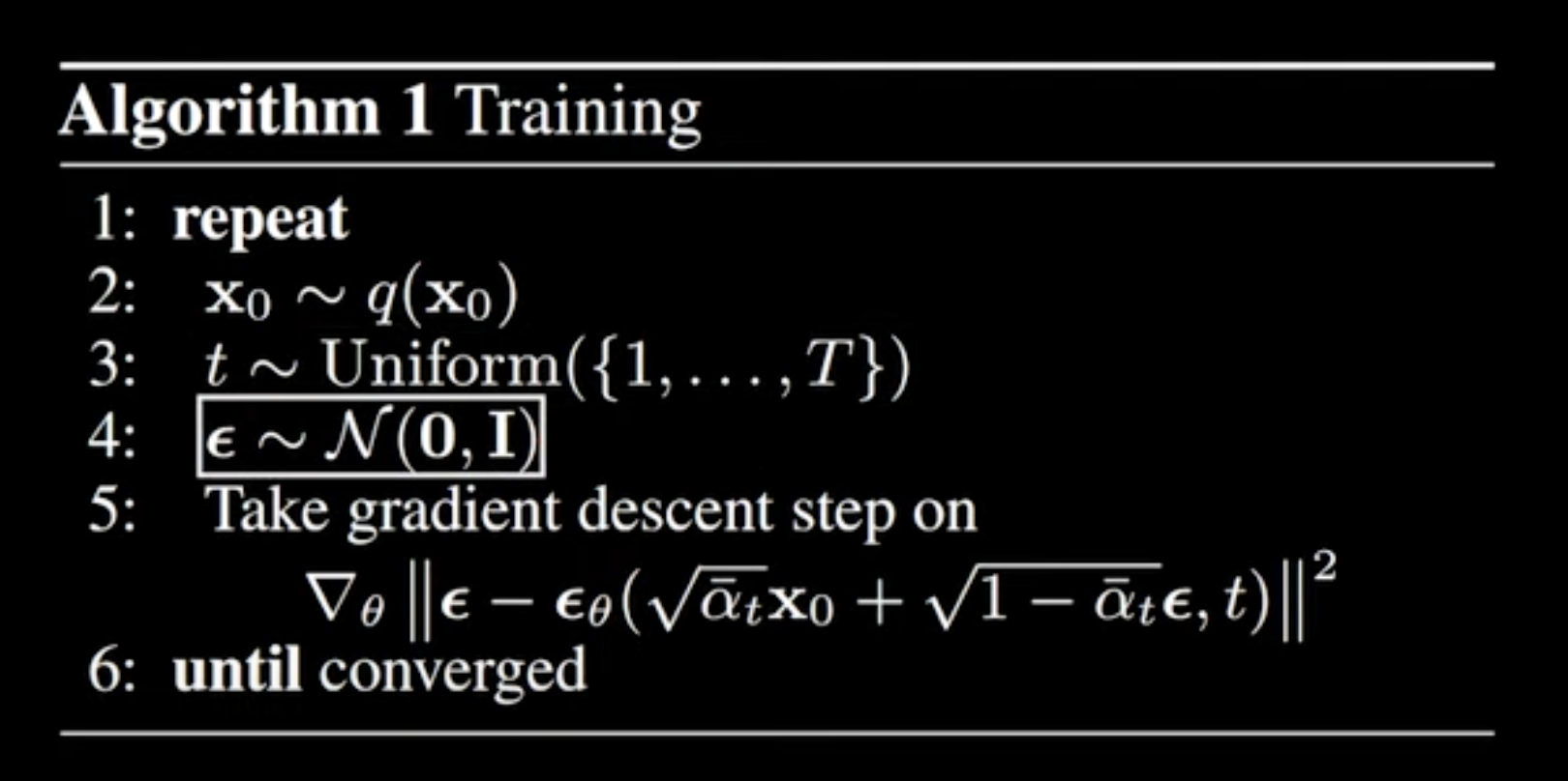
Outlier, Diffusion Models | Paper Explanation | Math Explained. (YouTube)
Sampling Algorithm
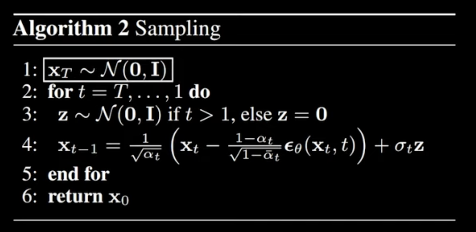
Outlier, Diffusion Models | Paper Explanation | Math Explained. (YouTube)
What This All Means
- The model is trained to match the true reverse dynamics of the noising process using KL divergence at each timestep.
- Instead of directly predicting \(x_0\), we train a model \(\epsilon_\theta(x_t, t)\) to predict the noise, and this enables us to recover the original data.
- The training loss simplifies to a weighted sum of per-timestep KL divergences, and with certain Gaussian assumptions, this becomes the familiar mean squared error loss:
Thus, diffusion models are likelihood-based models, unlike GANs.
- The reverse process is learned by minimizing the ELBO, typically using a simple squared error loss.
- The ELBO consists of:
- A reconstruction loss (like in VAEs)
- A KL divergence with the prior
- A sum of KL divergences at each timestep to match reverse distributions