
Background & Motivation
CLIP-based models are everywhere. They power image search, multimodal AI assistants, and zero-shot classifiers. They work by training a joint embedding space between images and text, so that a photo of a dog and the phrase "a dog playing in the snow" end up at the same point in vector space. The original paper achieves this at massive scale: 400 million image-text pairs scraped from the internet, vision transformers with hundreds of millions of parameters, and weeks of compute across hundreds of GPUs.
I wanted to understand the mechanism from the inside by training a version myself. There is a gap between understanding what a model does and understanding why it works, and that gap only closes when you directly experiment with it. Unfortunately, I do not have a data center. But I do have Modal credits. This reproduction uses the much more tractable Flickr30k dataset, off-the-shelf pretrained encoders, and costs a few dollars end-to-end on a single GPU. The goal is not to match OpenAI's numbers — I want to build real intuition for what contrastive learning is actually doing and show that the tooling available today makes reproducing landmark papers incredibly accessible.
There is a gap between understanding what a model does and understanding why it works. That gap only closes when you directly experiment with it.
The original CLIP paper[1] by Radford et al. (2021) demonstrated that a model trained on 400M image-text pairs from the internet could match the zero-shot accuracy of a supervised ResNet-50[3] on ImageNet, all without seeing a single labeled ImageNet example. The key ingredient is contrastive learning: instead of predicting a fixed set of class labels, the model learns a joint embedding space where matching image-text pairs are close together and non-matching pairs are far apart. This relies on self-supervised learning where no additional human supervision is needed as our data already has text captions.
What is contrastive learning?
Standard supervised models learn a mapping from inputs to a fixed set of labels. CLIP takes a different approach: it learns a shared embedding space for images and text. Both encoders independently compress their input into a vector of the same dimension. The training objective asks: given a batch of $N$ image-text pairs, can you tell which image belongs to which caption?
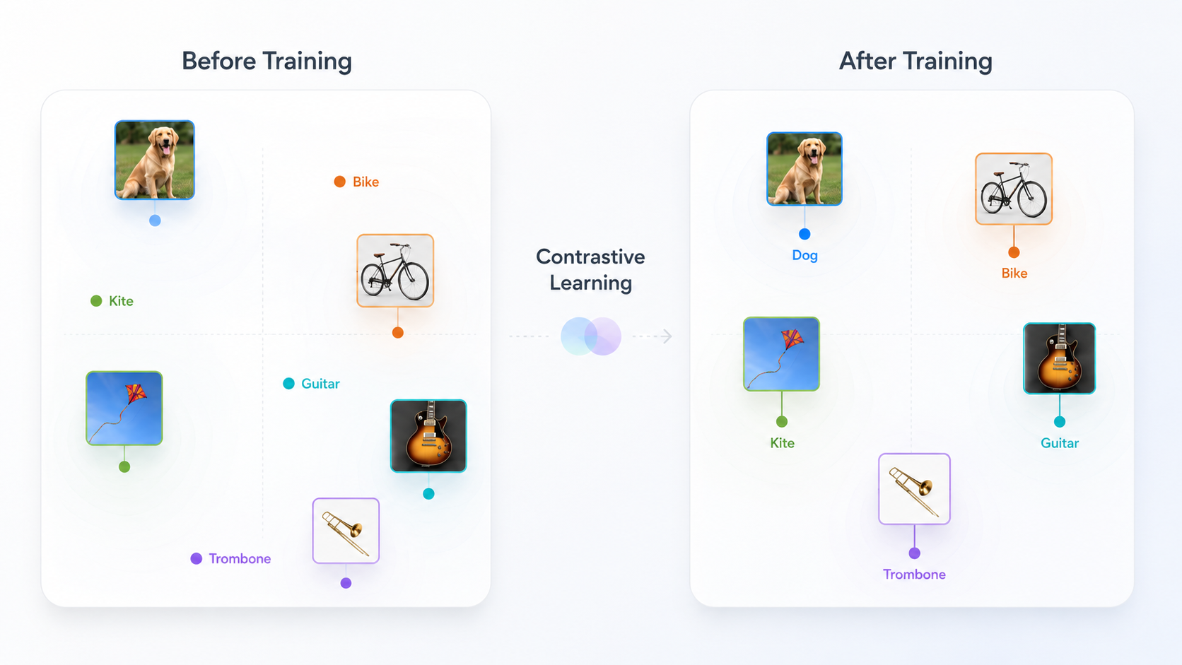
These comparisons are made across all image-text pairs in a batch of data. As an exercise, think about how training batch size affects performance of this model. After training on enough pairs, the embedding space develops a rich geometry so we can relate images and text.
The training objective
In each training step, we sample a batch of $N$ image-text pairs and compute all $N^2$ cosine similarities between image and text embeddings, forming an $N\times N$ matrix. The diagonal entries are the correct (positive) pairs; everything else is a negative. The loss asks the model to assign the highest similarity to each correct pair, for both images and text.
The best way to see this working is to watch the similarity matrix evolve during actual training. Each snapshot below is taken from my reproduction.
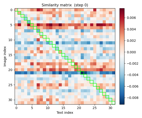
Beginning: uniform noise, diagonal indistinguishable.
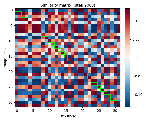
Mid-training: diagonal starts to emerge.
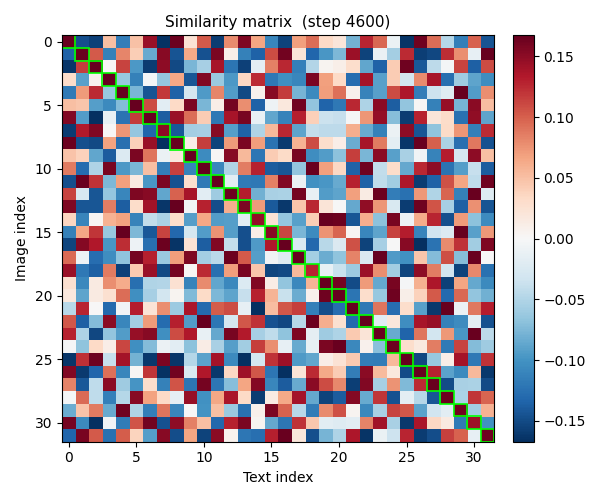
End of training: diagonal clearly dominant.
Model Architecture
Rather than training encoders from scratch — which requires hundreds of millions of pairs to work — I use pretrained architectures for each modality and let the contrastive objective teach them to agree on a shared coordinate system.
For images, I use ResNet[3] — a deep convolutional network built around residual connections. ResNet-18 and ResNet-50 are both pretrained on ImageNet, giving them rich visual representations out of the box. I replace the final classification head with a linear projection so the network outputs an embedding vector instead of class logits. Both encoders remain trainable throughout, so they fine-tune to the contrastive objective while retaining their pretrained features.
For text, the small model uses T5-small[5] (encoder only — the decoder is discarded) and the large model uses DistilBERT[4], a distilled version of BERT that retains 97% of its performance at 40% fewer parameters. Both are bidirectional transformers: every token attends to every other token in both directions, so mean-pooling over the final layer gives a genuinely global sentence representation.
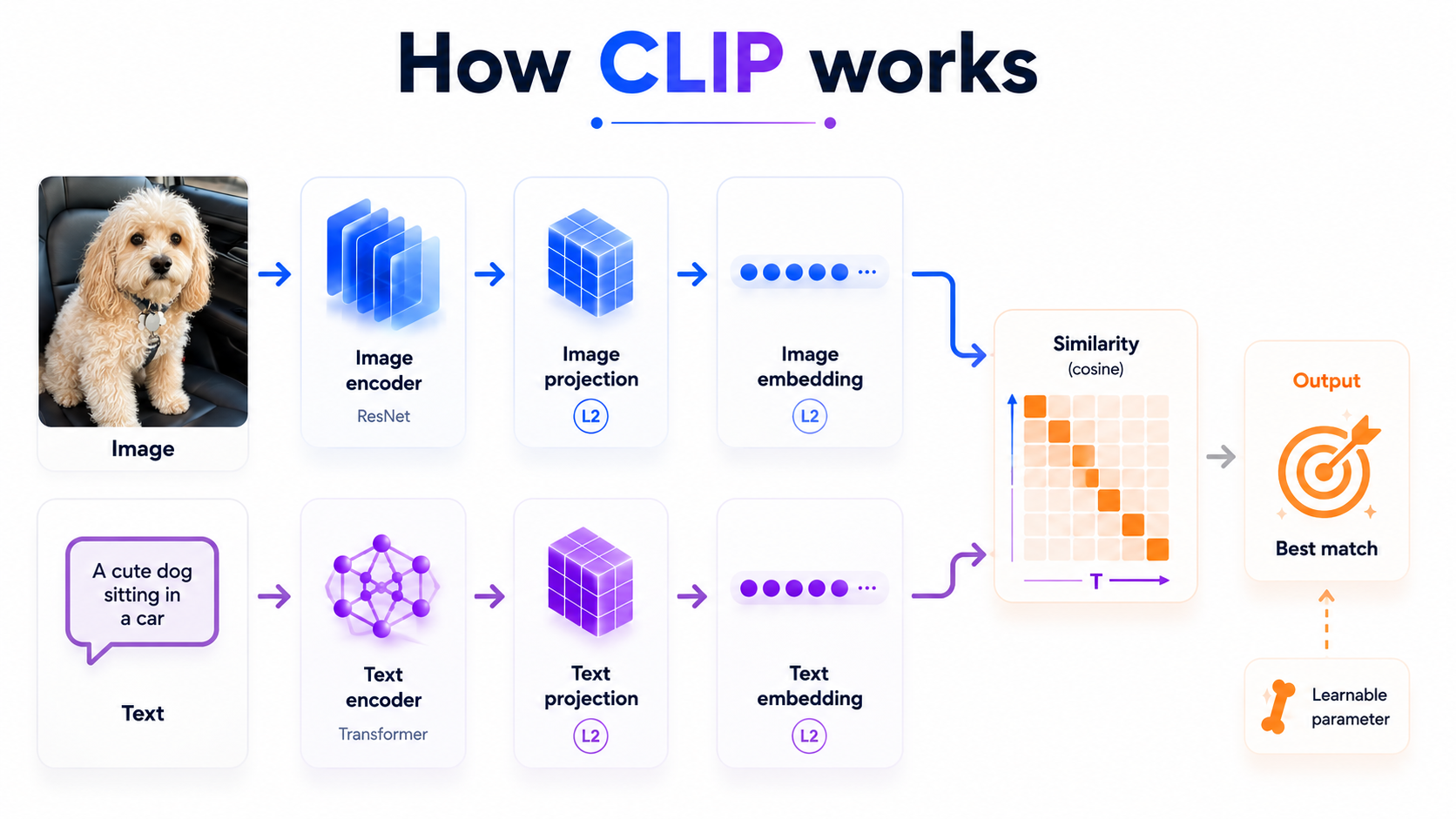
After encoding, a linear projection head (no bias) maps each encoder's output into a shared embedding space (256 dimensions for the small model and 512 for the large). Both embeddings are then L2-normalized: each vector is divided by its own magnitude so it lies on a unit hypersphere. This makes their dot product equal to cosine similarity, so similarity looks at the direction of embeddings.
Finally, the similarities are scaled by a learnable temperature parameter $\tau$. A small $\tau$ sharpens the softmax distribution, so the model becomes more decisive about which pair is correct. A large $\tau$ makes the distribution more uniform and the loss more forgiving.
Contrastive Loss
For a batch of $N$ image-text pairs, let $\mathbf{I}_i$ and $\mathbf{T}_i$ denote the L2-normalized image and text embeddings for pair $i$. Because both embeddings are unit vectors, their dot product equals their cosine similarity. The model scales these similarities by a learnable temperature $\tau$ and computes a symmetric cross-entropy loss over the resulting $N \times N$ logit matrix:
$$\mathcal{L} = -\frac{1}{2N} \sum_{i=1}^{N} \left[ \log \frac{\exp(\mathbf{I}_i \cdot \mathbf{T}_i \,/\, \tau)} {\sum_{j=1}^{N} \exp(\mathbf{I}_i \cdot \mathbf{T}_j \,/\, \tau)} \;+\; \log \frac{\exp(\mathbf{T}_i \cdot \mathbf{I}_i \,/\, \tau)} {\sum_{j=1}^{N} \exp(\mathbf{T}_j \cdot \mathbf{I}_i \,/\, \tau)} \right]$$The first term is the image-to-text direction: for each image $i$, treat its paired caption as the single correct class among all $N$ captions in the batch. The second term is the text-to-image direction: the same logic applied in reverse. Averaging the two makes the loss symmetric.
Dataset & Training Setup
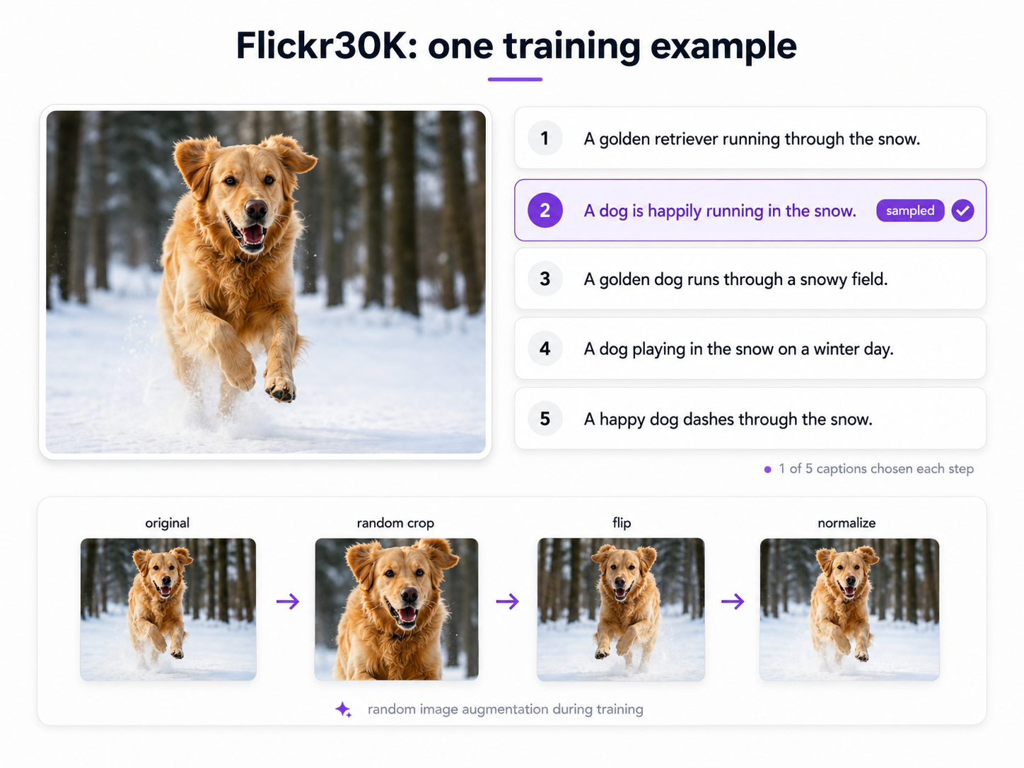
Flickr30k[2] contains 31,014 images, each with 5 independently-written human captions — 155,070 pairs in total. I hold out 1,000 images for validation and train on the remaining ~30,000. During training, one caption is sampled randomly per image per step, so the model sees different descriptions of the same scene across epochs, improving diversity without increasing dataset size. Images are randomly resized and cropped to 224 × 224, horizontally flipped with 50% probability, color-jittered, and normalized to ImageNet statistics for the pretrained ResNet.
| Hyperparameter | Value |
|---|---|
| Embedding dim | 256 (small) / 512 (large) |
| Batch size | 256 |
| Epochs | 40 |
| Optimizer | AdamW ($\beta_1 = 0.9$, $\beta_2 = 0.98$) |
| LR | 5e-4 (small) / 3e-4 (large) + Cosine annealing |
| Weight decay | 0.1 |
| Hardware | T4 (small) / A100 (large) via Modal |
| Training time | ~45 min (small) / ~1.5 hrs (large) |
The training and validation loss curves below show both models converging steadily over 40 epochs. The loss decreasing corresponds directly to the similarity matrix becoming more diagonal.
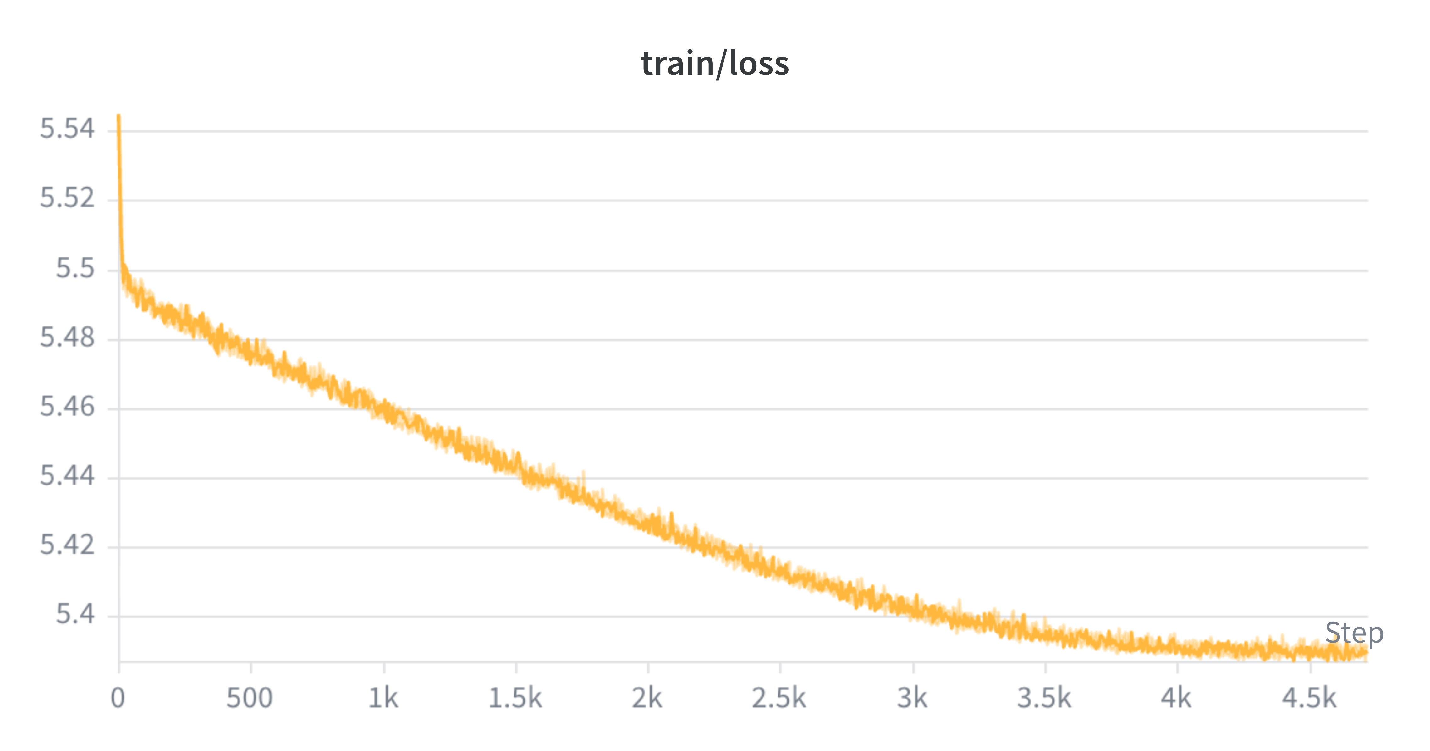
Training loss over 40 epochs
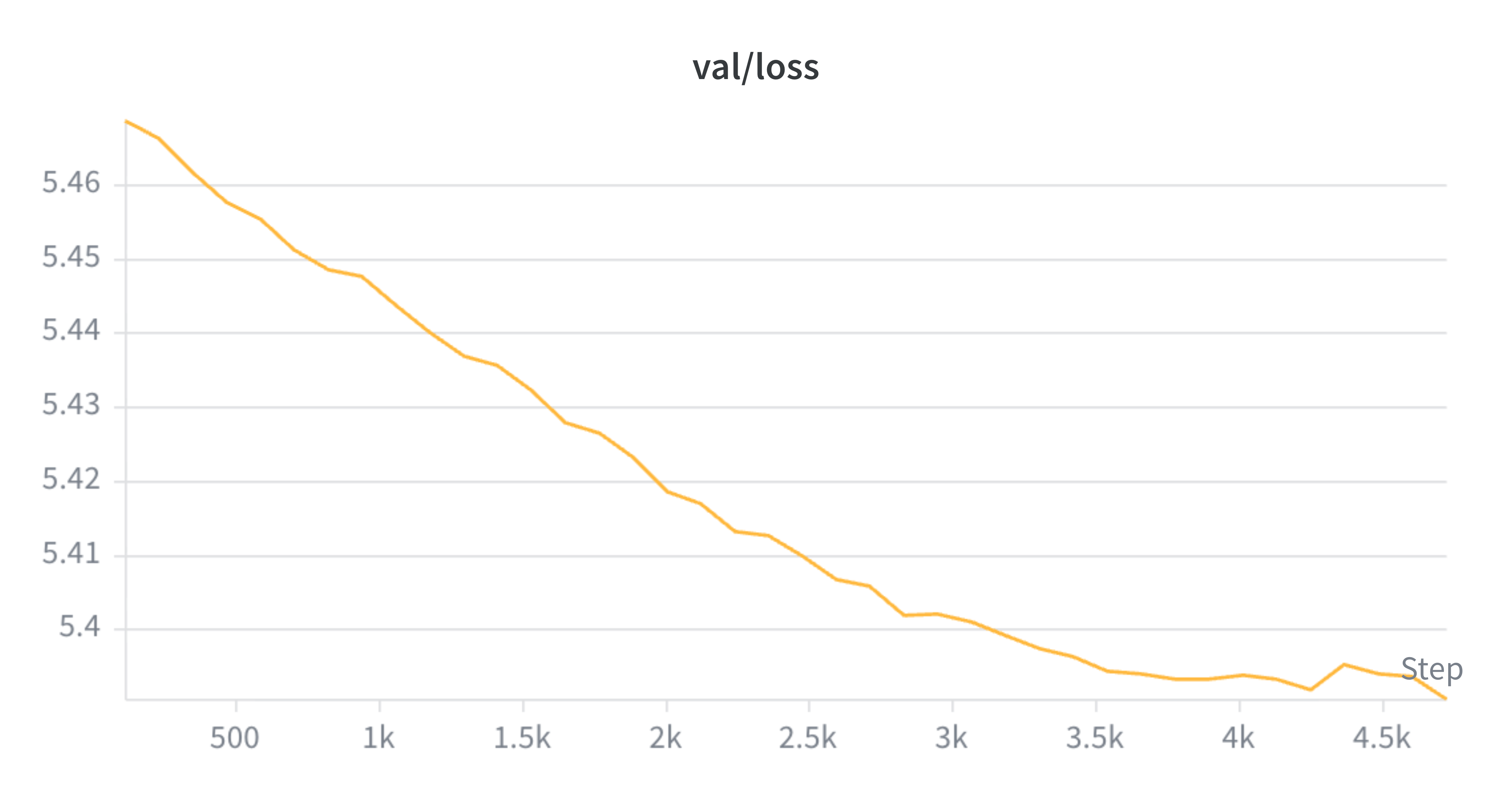
Validation loss over 40 epochs
Results
The primary evaluation metric for retrieval is Recall@$k$ (R@$k$): given a text query, is the correct image ranked in the top $k$ results out of 1,000 candidates? R@1 is the strictest since the model must pick the exact right image first. R@5 and R@10 are more forgiving, reflecting real-world use where a user scrolls through a few results.
Small model — T5-small + ResNet-18
Large model — DistilBERT + ResNet-50
The large model improves meaningfully across all metrics — R@1 goes from 1.9% to 5.2%, a 2.7× improvement just from scaling the encoders. Both are well below the original CLIP paper[1], which achieves R@1 = 88.0% on Flickr30k with a ViT-B/32 trained on 400M pairs. I don't expect to match that since they have 13,000× more data, a larger model, hundreds of GPUs, and weeks of training. The more meaningful comparison is random chance: with 1,000 candidates, random retrieval gives R@1 = 0.1%. The large model's 5.2% is 52× better than random, confirming the embedding space is learning a real structure.
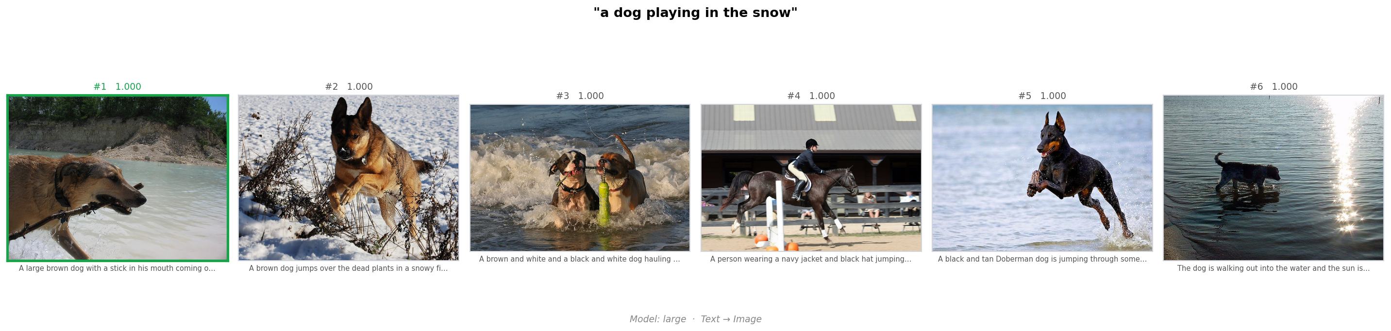
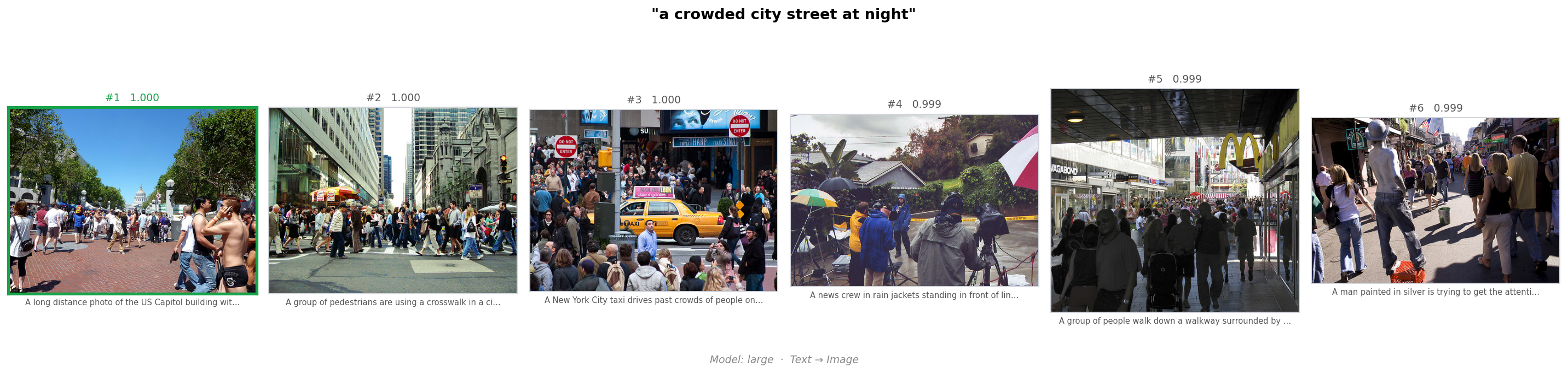
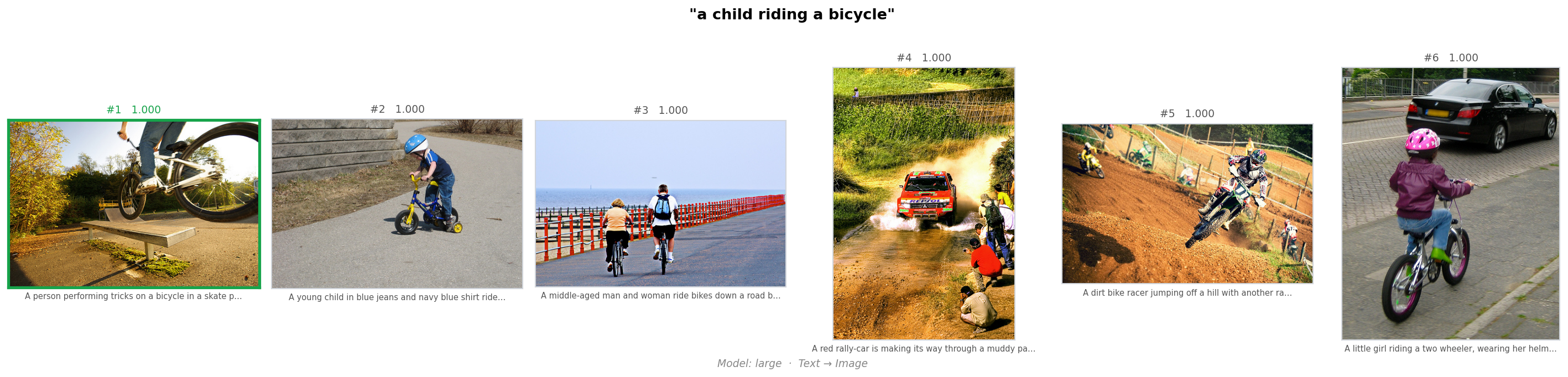
Retrieval Examples
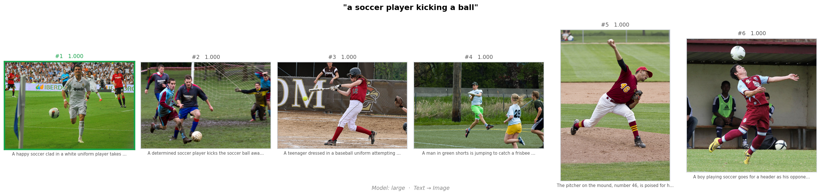
Given a text query, the model encodes it and retrieves the top-$k$ most similar images by cosine similarity across all 31,000 Flickr30k images. These results are from the large model (DistilBERT + ResNet-50). The top result (green border) is consistently relevant — the model has learned that images of active dogs (and a horse?) go with dog language, large groups of people go with crowded streets, and it can recognize a child riding a bike.
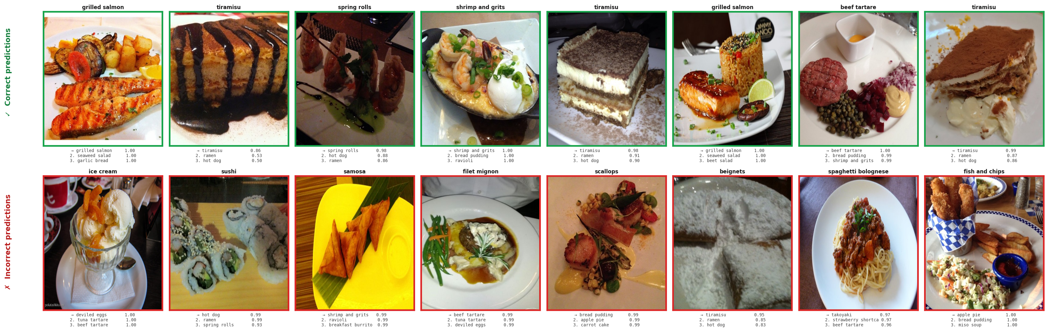
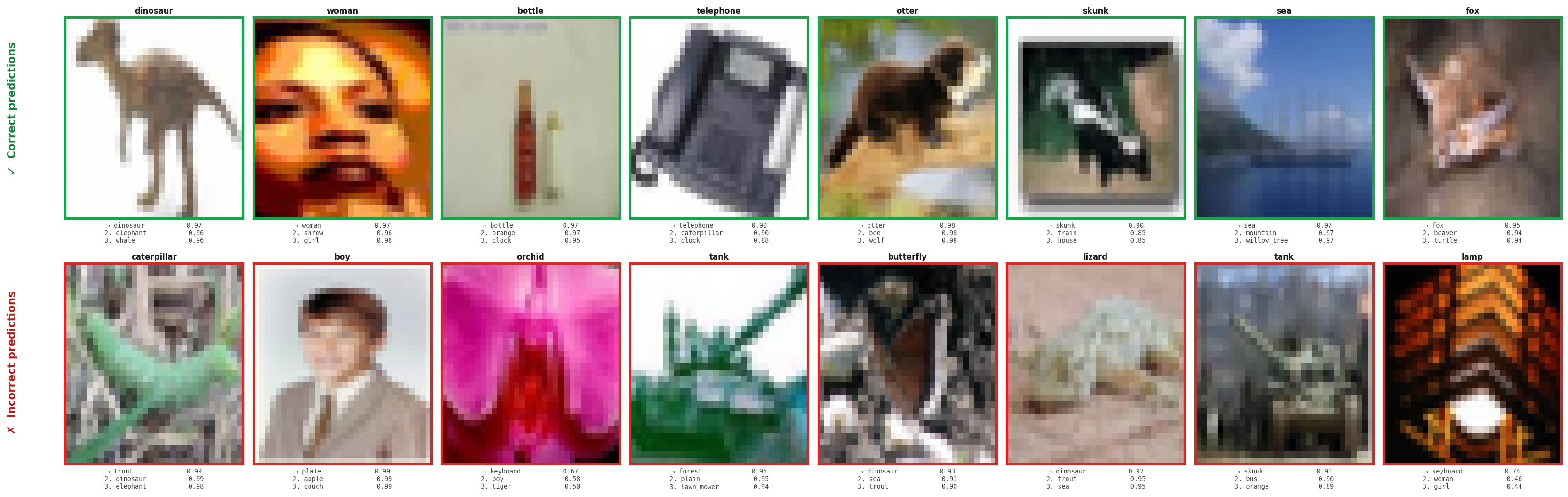
Zero-Shot Classification & Failure Cases
Beyond retrieval, CLIP's shared embedding space enables zero-shot classification: encode each class label as "a photo of a {class}", then find the nearest label to a query image, with no fine-tuning required. I tested both models on CIFAR-100 (100 fine-grained classes) and Food-101 (101 food categories).
The per-class breakdown reveals where the model succeeds and fails. On Food-101, visually distinctive categories (pizza, sushi, steak) score well. On CIFAR-100, fine-grained categories like shrew vs mouse or baby vs boy are nearly impossible. The 32×32 CIFAR images lose too much detail, and the model was never trained on anything like them.
Takeaways
The result that surprised me most: it works after 45 min. to 1 hr. of training. Training on 30,000 image-text pairs (a small dataset that fits in a few gigabytes that you can download in minutes) produces a model that can retrieve semantically relevant images from text queries. It can also generalize to zero-shot classification on datasets it never saw and produce a structured embedding space. That is not obvious and the contrastive objective is remarkably efficient at squeezing signal out of limited data.
The second surprise was how simple the implementation is. The core of CLIP fits in about 30 lines of Python: take two pretrained encoders, a linear projection, L2 normalization, a dot product, and a cross-entropy loss. There is no custom architecture and no complex pipeline. The pretrained encoders (ResNet and DistilBERT/T5) do the heavy lifting; the contrastive training just teaches them to agree. Plug in better encoders and more data and the same code scales up.
What the numbers also make clear is that data is the real bottleneck, not model capacity. Going from ResNet-18 to ResNet-50 and T5-small to DistilBERT gave a 2.7× improvement in R@1. But the gap to the original CLIP (which uses a similar model size) is 17× in R@1. That gap is almost entirely explained by training on 30K pairs vs 400M. More data would do more than any architectural change.
This might be my new favorite way to understand a paper. Reading CLIP gave me a clean mental model of what it does. Training it, watching the similarity matrix go from noise to structure, querying it with real text, and seeing it retrieve the right images and fail on hard cases gave me insight. I learned why it works and exactly where it breaks down and closed this gap in my mental model.
The tooling available today makes this surprisingly accessible. A GPU, a few dollars of cloud compute, some AI assistance, and a day or two is enough to reproduce the core of a landmark paper. That wasn't true five years ago. If you've been sitting on a paper you want to understand more deeply, the best next step is probably to just build it. Code available at github.com/ehersch/CLIP-blog.